What is Monte Carlo simulation?
Most spreadsheet models take one number for each input - the best guess - and return one number for the result. Real inputs are rarely that certain: a contractor's price could come in anywhere between two figures, a sales volume depends on the market, a task can run late. Monte Carlo simulation replaces each uncertain input with a probability distribution that describes the values it can take and how likely each one is.
The model is then recalculated many times - each recalculation is an iteration - with a fresh set of input values drawn from those distributions. After thousands of iterations you have thousands of possible results. Sorted and counted, they answer the questions a single estimate cannot: what is the chance of a loss, what budget is enough in 80% of cases, which input matters most.
The name comes from the casino in Monaco: the method uses random numbers, as a roulette wheel does, but in a controlled and repeatable way.
Why a single estimate is not enough
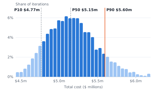
Adding up best guesses does not give the best guess of the total. Costs and durations are usually skewed - they can overrun far more than they can underrun - and risk events either happen or they do not. In the project cost model below, the sum of the most likely values is $4.83m, but the average simulated cost is $5.17m, $338k higher, and the single-point estimate is enough in only 15% of iterations.
How it works, step by step
- Build the model as usual. A spreadsheet that turns inputs into a result: costs into a total, cash flows into an NPV, durations into a finish date.
- Describe each uncertain input with a distribution. A three-point estimate (minimum, most likely, maximum) becomes a PERT or triangular distribution; a yes/no risk event becomes a Bernoulli; a fitted data series becomes the distribution that fits it best.
- Mark the outputs - the cells whose range you want to see.
- Run the iterations. For each one, draw a value for every input, let Excel recalculate, and record the outputs.
- Summarise. A histogram shows the shape of the results, a cumulative curve the probability of meeting any target, percentiles the key values and a tornado chart the inputs that drive the result.
A worked example in Excel
A capital project has four cost lines with three-point estimates and two risk events. In VionRisk (and in @RISK) each uncertain cell holds a distribution function; the total is an ordinary Excel formula wrapped with VROutput:
| Cell | Item | Formula |
|---|---|---|
| B1 | Design ($k) | =VRPert(420,480,610) |
| B2 | Civil works ($k) | =VRPert(1850,2100,2900) |
| B3 | Equipment ($k) | =VRTriang(1200,1300,1650) |
| B4 | Labour ($k) | =VRLognorm(950,140) |
| B5 | Ground risk occurs | =VRBernoulli(0.3) |
| B6 | Ground risk cost ($k) | =VRPert(150,300,700) |
| B7 | Permit delay occurs | =VRBernoulli(0.2) |
| B8 | Permit delay cost ($k) | =VRTriang(80,200,450) |
| B9 | Total cost ($k) | =VROutput("Total cost")+SUM(B1:B4)+B5*B6+B7*B8 |
Simulating it gives the distribution of total cost. Eight iterations in ten fall between the P10 of $4.77m and the P90 of $5.60m, and the median is $5.15m:
VionRisk 0.7.0 - 10,000 iterations, Latin Hypercube, seed 2026 · SVG
The full use case, with the S-curve for the contingency and the tornado chart of drivers, is on the use cases page.
Latin Hypercube vs Monte Carlo sampling
Plain Monte Carlo sampling draws every value independently at random. By chance, a run can over-sample one part of an input's range and miss another, and that noise shows up in the results.
Latin Hypercube sampling (LHS) splits each input's probability range into as many equal slices as there are iterations and draws exactly one value from each slice, in random order. Every part of every distribution is represented, so the results settle with fewer iterations. Both methods give the same answer on average; LHS has less noise around it. It is the default in VionRisk, as in @RISK.
The chart shows how far the estimated mean of the project cost moves from run to run, measured over 60 runs with different seeds at each number of iterations:
VionRisk 0.7.0 - project cost model, 60 seeds per point, Monte Carlo and Latin Hypercube · SVG
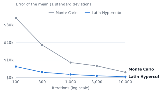
At 1,000 iterations the mean from Monte Carlo sampling moves by about $8.6k (one standard deviation) between runs; with Latin Hypercube it moves by $1.8k. Latin Hypercube at 300 iterations ($3.1k) is about as steady as Monte Carlo at 10,000 ($3.0k). The gain is largest for the mean and for models where the inputs add up; it is smaller for extreme percentiles.
How many iterations?
Enough that the number you report stops moving. Three rules of thumb:
- The error of a mean shrinks with the square root of the iterations. For plain Monte Carlo the standard error is the standard deviation divided by √n: four times the iterations halves the error. For the cost model, a standard deviation of $320k over 10,000 iterations gives $3.2k.
- Percentiles need more than means, tails need more than percentiles. A P90 rests on the 10% of iterations above it; a 1-in-200 event on 0.5%. 5,000 to 10,000 iterations are common for P90 budgets; rare events need more, or a model of the tail itself.
- Fix the seed when you compare. With the same seed, two runs of the same model give identical results, and the difference between two versions of a model comes from the change, not from sampling noise. VionRisk records the seed with every result.
Reading the results
- Histogram - the shape: where results cluster, how long the tails are, whether there are two humps (often a risk event that either happens or not).
- Cumulative curve (S-curve) - the probability that the result is at or below any value. Read across from 80% to find the P80 budget; read up from a target to find its chance.
- Percentiles - P10, P50 (the median) and P90 are the common summary; P80 is a usual confidence level for budgets and contingencies.
- Mean vs median - for skewed results the mean sits above the median; the mean is what you pay on average across many projects, the median what a single project most often comes close to.
- Tornado chart - the inputs ranked by how strongly they move the output. It tells you where better information or a mitigation pays off.
- Correlation - if inputs move together in reality (price and volume, labour and materials), say so in the model; leaving correlation out can understate or overstate the risk. See the NPV example.
How to make a tornado chart in Excel
A tornado chart for a simulation ranks the inputs by their rank (Spearman) correlation with the output. With VionRisk it is one click: Results > Sensitivity, or the Sensitivity report. To build one by hand in Excel:
- Collect the iterations. One row per iteration, one column per uncertain input and one for the output. A simulation add-in writes these for you; in plain Excel, a one-variable Data Table that recalculates a RAND-based model gives the same table.
- Rank every column. Next to the data, use
=RANK.AVG(B2,B$2:B$10001,1), filled down and across, so ties get the average rank. - Correlate the ranks. For each input,
=CORREL(rank of the input,rank of the output)is its Spearman rank correlation with the output. - Sort by size. Copy the names and correlations to a small table, add
=ABS()of each correlation and sort by it, largest first. - Insert a bar chart. Select the names and correlations and insert a clustered bar chart. Format the vertical axis with Categories in reverse order so the largest bar is on top, and fix the horizontal axis from -1 to 1.
- Label and read it. Add data labels, remove the legend, and title the chart with the finding. Bars to the right raise the output as the input rises; bars to the left lower it.
The result for the project cost model, from VionRisk's sensitivity analysis:
VionRisk 0.7.0 - 10,000 iterations, Latin Hypercube, seed 2026 · SVG
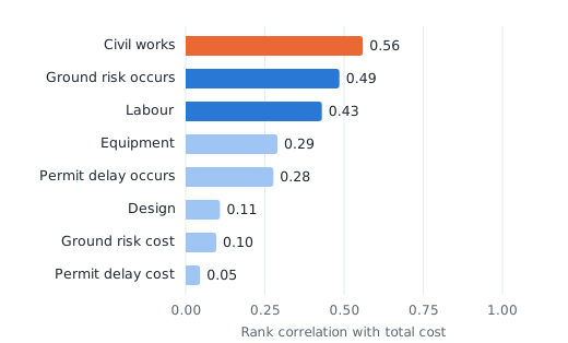
Rank correlation measures association in the simulated data, not proven cause: an input can rank high because it is correlated with another one that matters. VionRisk also offers regression coefficients, contribution to variance and the change in the output's mean across each input's range (the default in @RISK's tornado).
Monte Carlo in plain Excel, without an add-in
You can run a simple simulation with Excel's own functions:
- Draw a normal value with
=NORM.INV(RAND(),mean,sd), a lognormal with=LOGNORM.INV(RAND(),mu,sigma), and a yes/no event with=IF(RAND()<p,1,0). - Put the iteration numbers 1 to 10,000 in a column, point a one-variable Data Table (What-If Analysis > Data Table) at the output, and Excel recalculates the model once per row.
- Summarise with
PERCENTILE.INC,AVERAGE, a histogram chart and the tornado steps above.
This works for small models and is a good way to learn. Its limits show quickly: RAND() cannot be seeded, so results change on every recalculation; there is no PERT, triangular or fitted distribution built in; correlation between inputs takes extra work; Latin Hypercube sampling is not available; large Data Tables are slow; and the results are a table of numbers, not a report. A simulation add-in handles these for you - VionRisk with the same worksheet functions as @RISK, so existing models run as they are.
Questions
What is Monte Carlo simulation?
Monte Carlo simulation is a way to see the range of possible outcomes of a model whose inputs are uncertain. Each uncertain input is described by a probability distribution; the model is recalculated thousands of times with values drawn from those distributions, and the collected results show how likely each outcome is.
Can you do Monte Carlo simulation in Excel?
Yes. In plain Excel you can draw random values with RAND() and inverse distribution functions such as NORM.INV(RAND(),mean,sd) and repeat the calculation with a Data Table. A simulation add-in such as VionRisk adds ready-made distributions, Latin Hypercube sampling, correlation, a fixed seed, and charts and reports of the results.
What is the difference between Latin Hypercube and Monte Carlo sampling?
Plain Monte Carlo draws every value independently at random. Latin Hypercube sampling splits each input's probability range into as many equal slices as there are iterations and draws exactly once from each slice, so the whole range is covered evenly. Both give the same answer on average; Latin Hypercube gets there with fewer iterations.
How many iterations does a Monte Carlo simulation need?
Enough that the statistic you report stops moving. For the mean, the error of plain Monte Carlo shrinks with the square root of the number of iterations, so four times the iterations halves it. 1,000 iterations are often enough for a mean with Latin Hypercube sampling; 5,000 to 10,000 are common for percentiles such as P90, and more for rare tail events.
What do P10, P50 and P90 mean?
They are percentiles of the simulated results: P10 is the value that 10% of iterations fall below, P50 the median and P90 the value that 90% fall below. A P80 budget is a budget that is enough in 80% of the iterations.
Run your own model
VionRisk runs existing @RISK workbooks unchanged and explains the results with AI agents. Try it on one of your models in a pilot.